Transformer 基础

Attention

Scaled Dot-product Attention 点积注意力机制

在注意力机制里，有三个关键向量

Query 当前要关注的对象
Key 候选信息的索引
Value 真正的信息内容

目的：让 Query 去匹配 Key，找到相关的 Value

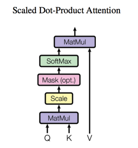
首先 Q 和 K 相乘，假设 Q 是长度为 $m$ 的序列，K 是长度为 $n$ 的序列，运算完成之后生成了一个尺寸为 $m \times n$ 的注意力分数矩阵 score

然后缩放 Scale，把 score 除以 $\sqrt{d_{k}}$

然后对每一行所 softmax 得到 $w_{i, j}$ 表示第 $i$ 个 query 向量和第 $j$ 个 key 向量之间的关联程度

最后更新 token embeddings 将 $w_{i, j}$ 与对应的 value 向量 $v_{1}, v_{2}, \dots, v_{n}$ 相乘获得第 $i$ 个 query 向量更新后的语言，表示为 $x_{i}^{'} = \sum_{j} w_{i, j} v_{j}$

用公式表示为

Attention(Q,K,V) = softmax (\frac{Q K^{T}}{\sqrt{d_{k}}}) V

接下来尝试用代码去实现一下 Scaled Dot-product Attention

首先需要将文本分词为词语（token）序列，然后将每一个词语转换为对应的词向量（embedding）

from torch import nn
from transformers import AutoConfig, AutoTokenizer

model_ckpt = 'bert-base-uncased' # 指定使用预训练语言模型 BERT-base
tokenizer = AutoTokenizer.from_pretrained(model_ckpt) # 加载分词器

text = 'time flies like an arrow'

# 分词并转换为张量
# return_tensors='pt' 表示返回 PyTorch 张量
# add_special_tokens=True 表示添加特殊标记（如 [CLS] 和 [SEP]
inputs = tokenizer(text, return_tensors='pt', add_special_tokens=True) 
print(inputs.input_ids) # 输出张量的 input_ids 部分

config = AutoConfig.from_pretrained(model_ckpt) # 加载模型配置，词表大小为 vocab_size，嵌入维度为 hidden_size
token_emb = nn.Embedding(config.vocab_size, config.hidden_size) # 创建嵌入层
print(token_emb) # 输出嵌入层信息

inputs_embeds = token_emb(inputs.input_ids) # 将 input_ids 转换为嵌入表示
print(inputs_embeds.shape) # 输出嵌入表示的形状 (batch_size, sequence_length, hidden_size)

tensor([[ 101, 2051, 10029, 2066, 2019, 8612, 102]]) 
Embedding(30522, 768)
torch.Size([1, 7, 768])

可以看到 BERT-base-uncased 模型对应的词表大小为 30522,每个词语的词向量纬度为 768，Emdding 层把输入的词语序列映射到了尺寸为 [betch_size, seq_len, hidden_dim] 的向量，在这里就是 [1,7, 768]

接下来就是创建向量序列 $Q, K, V$ 了，并且要使用点积作为相似度函数来计算注意力分数

import torch
from math import sqrt

Q = K = V = inputs_embeds # 在 BERT 模型中，Q,K,V 都是一样的
dim_k = K.size(-1)
# 批量矩阵乘法
# Q : [batch_size, seq_len, dim_k]
# K : [batch_size, seq_len, dim_k]
# scores : [batch_size, seq_len, seq_len]
scores = torch.bmm(Q, K.transpose(1, 2)) / sqrt(dim_k) 
print(scores.size())

torch.Size([1, 7, 7])

softmax 层

import torch.nn.functional as F

weights = F.softmax(scores, dim=-1) # 计算注意力权重
print(weights.size())
print(weights.sum(dim=-1)) # 输出注意力权重

torch.Size([1, 7, 7])
tensor([[1., 1., 1., 1., 1., 1., 1.]], grad_fn=<SumBackward1>)

attn_output = torch.bmm(weights, V) # 计算注意力输出
print(attn_output.size()) # 输出注意力输出的形状 (batch_size, seq

torch.Size([1, 7, 768])

至此，就实现了一个简化版的 Scaled Dot-product Attention，把上面的操作封装为函数以后方便后续调用

import torch
import torch.nn.functional as F
from math import sqrt

def scaled_dot_product_attention(query, key, value, query_mask=None, key_mask=None, mask=None):
    dim_k = query.size(-1)
    scores = torch.bmm(query, key.transpose(1, 2)) / sqrt(dim_k)
    if query_mask is not None and key_mask is not None:
        mask = torch.bmm(query_mask.unsqueeze(-1), key_mask.unsqueeze(1))
    if mask is not None:
        scores = scores.masked_fill(mask == 0, -float("inf"))
    weights = F.softmax(scores, dim=-1)
    return torch.bmm(weights, value)

上述代码中海考虑了 Mask，填充的字符的注意力 scores 被设置为 $- \infty$

这样的做法会带来一个问题，当 $Q = K$ 的时候，注意力机制会为上下文中的相同单词分配非常大的分数，点积为 $1$ ，但实际上，相关词往往比相同词更重要

所以。多头注意力机制 Multi-head Attention 出现了

Multi-head Attention

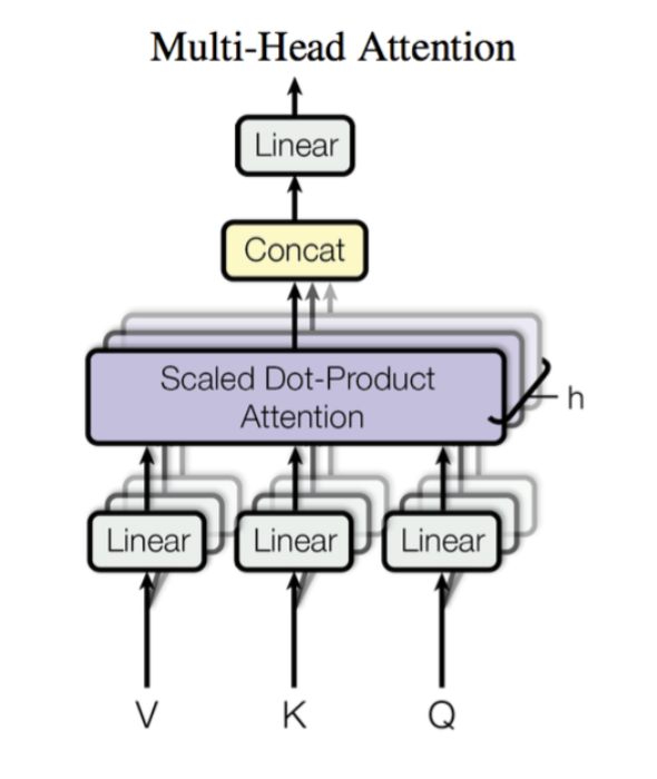
Multi-head Attention 首先通过线性映射将 $Q, K, V$ 序列映射到特征空间，每一组线性投影后到向量称为一个头（head），然后在每组映射后的序列上再应用 Scaled Dot-product Attention

每个注意力头负责关注某一方面的语义相似性，多个头就可以让模型同时关注多个方面。因此与简单的 Scaled Dot-product Attention 相比，Multi-head Attention 可以捕获到更加复杂的特征信息。

\begin{array}{r} {head}_{i} = Attention (Q W_{i}^{Q}, K W_{i}^{K}, V W_{i}^{V}) \\ MultiHead (Q, K, V) = Concat ({head}_{1}, \dots, {head}_{h}) \end{array}

来尝试实现一个多头注意力机制，首先实现一个注意力头：

from torch import nn

class AttentionHead(nn.Module):
    def __init__(self, embed_dim, head_dim):
        super().__init__()
        self.q = nn.Linear(embed_dim, head_dim)
        self.k = nn.Linear(embed_dim, head_dim)
        self.v = nn.Linear(embed_dim, head_dim)

    def forward(self, query, key, value, query_mask=None, key_mask=None, mask=None):
        attn_outputs = scaled_dot_product_attention(
            self.q(query), self.k(key), self.v(value), query_mask, key_mask, mask
        )
        return attn_outputs

每个头都会初始化三个独立的线性层，负责将 $Q, K, V$ 序列映射到尺寸为 [batch_size, seq_len, head_dim] 的张量

然后拼接多个注意力头的输出就可以构建出 Multi-head Attention 了

然后把拼接后的张量做一个线性变换来生成最终的张量

class MultiHeadAttention(nn.Module):
    def __init__(self, config):
        super().__init__()
        embed_dim = config.hidden_size # 词向量的维度
        num_heads = config.num_attention_heads # 多头注意力机制中的头数
        head_dim = embed_dim // num_heads # 每个头的维度
        self.heads = nn.ModuleList(
            [AttentionHead(embed_dim, head_dim) for _ in range(num_heads)]
        )
        self.output_linear = nn.Linear(embed_dim, embed_dim) # 输出线性层

    def forward(self, query, key, value, query_mask=None, key_mask=None, mask=None):
        # 拼接所有头的输出
        x = torch.cat([
            head(query, key, value, query_mask, key_mask, mask) for head in self.heads
        ], dim=-1)
        x = self.output_linear(x) # 通过输出线性层
        return x

这里使用 BERT-base-uncased 模型的参数初始化 Multi-head Attention 层，并且将之前构建的输入送入模型以验证是否正常工作

from transformers import AutoConfig
from transformers import AutoTokenizer

model_ckpt = 'bert-base-uncased' # 指定使用预训练语言模型 BERT-base
tokenizer = AutoTokenizer.from_pretrained(model_ckpt) # 加载分词器

text = 'time flies like an arrow'
inputs = tokenizer(text, return_tensors='pt', add_special_tokens=True) # 分词并转换为张量
config = AutoConfig.from_pretrained(model_ckpt) # 加载模型配置
token_emb = nn.Embedding(config.vocab_size, config.hidden_size) # 创建 embedding 层
inputs_embeds = token_emb(inputs.input_ids) # 将 input_ids 转换为 embedding 表示

multihead_attn = MultiHeadAttention(config) # 创建多头注意力机制
query = key = value = inputs_embeds # 在 BERT 模型中，Q,K,V 都是一样的
attn_output = multihead_attn(query, key, value) # 计算多头

print(attn_output.size()) # 输出多头注意力输出的形状 (batch_size, seq_len, embed_dim)

torch.Size([1, 7, 768])

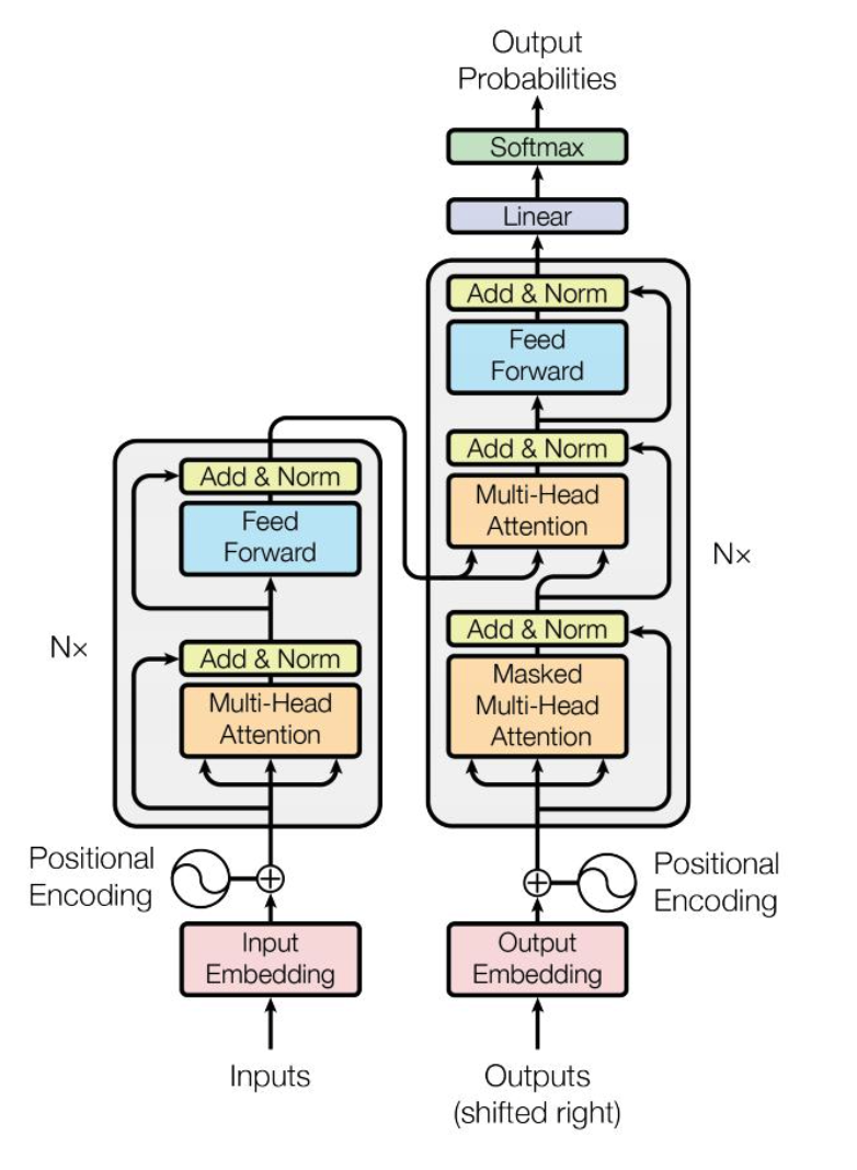
Encoder

回顾一下 Transformer 的基本结构，Encoder 复杂将输入的词语序列转化成词向量序列，

Decoder 则基于 Encoder 的隐状态来迭代地生成词语序列作为输出，每次生成一个词语

来看一个翻译的任务

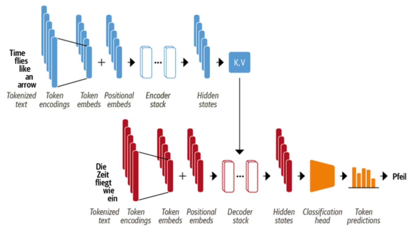
输入的词语首先被转换为词向量。由于注意力机制无法捕获词语之间的位置关系，因此还通过 positional embeddings 向输入中添加位置信息；
Encoder 由一堆 encoder layers 组成，同样的，Decoder 里面也包含有堆叠的 decoder layers
Encoder 的输出被送入到 Decoder 层中以预测概率最大的下一个词，然后当前的词语序列又被送回到 Decoder 中以继续生成下一个词，重复直至出现序列结束符 EOS 或者超过最大输出长度。

The Feed-Forward Layer

Transformer Encoder/Decoder 中的前馈子层实际上就是两层全连接神经网络，它单独地处理序列中的每一个词向量，也被称为 position-wise feed-forward layer。常见做法是让第一层的维度是词向量大小的 4 倍，然后以 GELU 作为激活函数。

下面实现一个简单的 Feed-Forward Layer：

class FeedForward(nn.Module):
    def __init__(self, config):
        super().__init__()
        self.linear_1 = nn.Linear(config.hidden_size, config.intermediate_size)
        self.linear_2 = nn.Linear(config.intermediate_size, config.hidden_size)
        self.gelu = nn.GELU()
        self.dropout = nn.Dropout(config.hidden_dropout_prob)

    def forward(self, x):
        x = self.linear_1(x)
        x = self.gelu(x)
        x = self.linear_2(x)
        x = self.dropout(x)
        return x

将前面注意力层的输出送入到该层中以测试是否符合我们的预期

feed_forward = FeedForward(config)
ff_outputs = feed_forward(attn_output)
print(ff_outputs.size())

torch.Size([1, 7, 768])

Layer Normalization

Layer Normalization 负责将一批 (batch) 输入中的每一个都标准化为均值为零且具有单位方差；

Skip Connections 则是将张量直接传递给模型的下一层而不进行处理，并将其添加到处理后的张量中。

向 Transformer Encoder/Decoder 中添加 Layer Normalization 目前共有两种做法

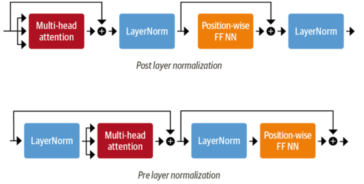
Post layer normalization：Transformer 论文中使用的方式，将 Layer normalization 放在 Skip Connections 之间。但是因为梯度可能会发散，这种做法很难训练，还需要结合学习率预热 (learning rate warm-up) 等技巧；

Pre layer normalization：目前主流的做法，将 Layer Normalization 放置于 Skip Connections 的范围内。这种做法通常训练过程会更加稳定，并且不需要任何学习率预热。

下面采用第二种方式来构建 Transformer Encoder 层

class TransformerEncoderLayer(nn.Module):
    def __init__(self, config):
        super().__init__()
        self.layer_norm_1 = nn.LayerNorm(config.hidden_size)
        self.layer_norm_2 = nn.LayerNorm(config.hidden_size)
        self.attention = MultiHeadAttention(config)
        self.feed_forward = FeedForward(config)

    def forward(self, x, mask = None):
        # 第一个子层：多头注意力机制 + 残差连接 + 层归一化
        hidden_states = self.layer_norm_1(x)
        x = x + self.attention(hidden_states, hidden_states, hidden_states, mask=mask)

        # 第二个子层：前馈网络 + 残差连接 + 层归一化
        hidden_states = self.layer_norm_2(x)
        x = x + self.feed_forward(hidden_states)
        return x

同样的，这里将之前构建的层输入到该层中进行测试

encoder_layer = TransformerEncoderLayer(config) # 创建 Transformer encoder层
print(inputs_embeds.shape)
print(encoder_layer(inputs_embeds).shape)

torch.Size([1, 7, 768])
torch.Size([1, 7, 768])

Positional Embeddings

注意力机制无法捕捉词语之间的位置信息，因此我们使用了 Positional Embeddings 添加了词语的位置信息

Position Embeddings 的方法很多，一种常见的做法是把词语的位置映射到一个位置向量上面，然后把位置向量和词向量相加，就是最终的输出

class Embeddings(nn.Module):
    def __init__(self, config):
        super().__init__()
        # 词嵌入层 从词的 token id 映射到一个词向量
        self.token_embeddings = nn.Embedding(config.vocab_size, config.hidden_size)
        # 位置 embedding 层
        # 每个位置 id 对应一个位置向量
        self.position_embeddings = nn.Embedding(config.max_position_embeddings, config.hidden_size)
        self.layer_norm = nn.LayerNorm(config.hidden_size, eps=1e-12)
        self.dropout = nn.Dropout()

    def forward(self, input_ids):
        seq_length = input_ids.size(1) # 序列长度
        position_ids = torch.arange(seq_length, dtype=torch.long).unsqueeze(0) # 位置 id
        token_embeddings = self.token_embeddings(input_ids) # 获得每个词的词向量
        position_embeddings = self.position_embeddings(position_ids) # 获得每个位置的向量
        embeddings = token_embeddings + position_embeddings # 将词向量和位置向量相加
        embeddings = self.layer_norm(embeddings) # 层归一化
        embeddings = self.dropout(embeddings) # dropout
        return embeddings
    
embedding_layer = Embeddings(config)
print(embedding_layer(inputs.input_ids).shape)

torch.Size([1, 7, 768])

除此之外，Position Embeddings 还有其他的做法

之后我们把这些层结合起来就是完整的 Transformer Encoder

class TransformerEncoder(nn.Module):
    def __init__(self, config):
        super().__init__()
        self.embeddings = Embeddings(config) # 词嵌入层
        self.layers = nn.ModuleList([
            TransformerEncoderLayer(config) for _ in range(config.num_hidden_layers)
        ]) # 多个 Transformer encoder 层

    def forward(self, input_ids, mask=None):
        x = self.embeddings(input_ids)
        for layer in self.layers:
            x = layer(x, mask=mask)
        return x

encoder = TransformerEncoder(config)
print(encoder(inputs.input_ids).shape)

torch.Size([1, 7, 768])

Transformer Decoder

Transformer Decoder 和 Encoder 的最大不同是有两个注意力子层

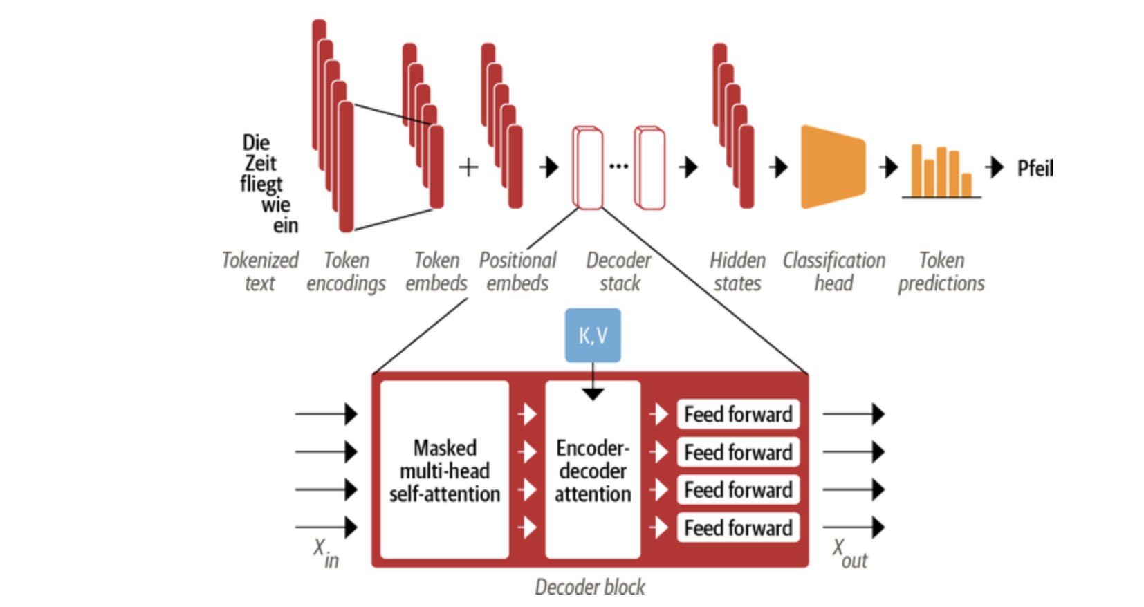
Masked multi-head self-attention layer：掩码注意力机制确保在每个时间步生成的词语仅基于过去的输出和当前预测的词

Encoder-decoder attention layer：以 Encoder 的输出作为 queries，对 key 和 value 向量执行 Muti-head Attention